
How households self-insure against job loss
Asger Lau Andersen, Amalie Jensen, Niels Johannesen, Claus Thustrup Kreiner, Søren Leth-Petersen, Adam Sheridan
To what extent do households self-insure to avoid cutting back on consumption following income losses, and which self-insurance channels are most important?
This column reviews evidence on household responses to job loss using comprehensive high-frequency data from multiple sources in Denmark. Over the two years following job loss, 30% of the decline in disposable income is accounted for by a drop in household spending, leaving a gap of 70% that reflects the effects of self-insurance. This gap is filled by lower accumulation of liquid assets (~50%), increases in private transfers and other inflows (~10%), higher spousal labour supply (~5%), and lower net debt repayments (~5%). Mortgage borrowing and refinancing play only a small role.
Losing a job causes a significant and persistent drop in disposable income for the average household, despite the existence of extensive unemployment insurance programmes in many countries (e.g. Jacobson et al. 1993, Flaaen et al. 2019). Several studies document that consumption also drops following job loss, but by much less (e.g. Jappelli and Pistaferri 2010, Ganong and Noel 2019, Landais and Spinnewijn 2020). This suggests that households partially self-insure against the adverse consequences of job loss, but how they do so remains an open question.
Various self-insurance mechanisms have been analysed in the literature. Households can compensate for the lost income through an increase in spousal labour supply (Halla et al. 2018, De Nardi et al. 2020) or transfers from family and friends (McGarry 2016). They can refinance their mortgages (Cocco 2013) or take up consumer loans (Sullivan 2008), or they can tap into their holdings of liquid assets (Basten et al. 2016).
The relative importance of these responses is hard to assess. Existing studies typically focus on a single response margin, and samples, data types, and research designs vary across studies, making comparisons difficult.
In our new research (Andersen et al. 2020), we overcome this problem by analysing all of these self-insurance responses ‒ as well as the effects on income and spending ‒ in a unified framework, using the same sample of households, the same definition of job loss, and the same research design. While existing studies typically rely on annual data, we study all these margins at the monthly frequency, providing more compelling identification of the various effects.
High-frequency data from multiple sources
We merge transaction-level data from the largest bank in Denmark with administrative data from multiple government registers. From tax registers, we match employer-employee payroll data as well as monthly information about unemployment insurance (UI) benefits recipience, which allows us to infer the timing of job losses with high precision. From the population register, we observe household structures. Combining this with the detailed transaction data, we can construct monthly household-level measures of disposable income, spending, saving, and borrowing.
On the income side, we can separate salary payments, government income transfers, and private transfers (including transfers from family and friends) and distinguish salary payments to the person losing a job from those to the spouse. Note that this is only possible due to the unique combination of data sources.
The resulting dataset covers all the behavioural responses mentioned above. Crucially, our estimates of these responses add up to match the drop in disposable income almost perfectly, suggesting that we capture all empirically relevant margins.
Figure 1 shows the dynamics of key variables on a timeline centred on the month of job loss, illustrating how each of them is affected by the job loss. All variables are measured relative to monthly disposable income in the months before job loss.
Figure 1 Income, spending, and self-insurance responses to job loss
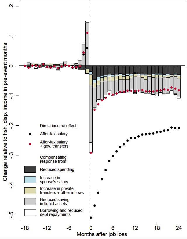 Note: All outcomes measured relative to the household’s average disposable income in the months before the job loss.
Impact on income
Job loss has a large effect on the affected person’s after-tax salary income (black dots in Figure 1). Salary payouts are higher than normal in the two months before job loss, due to sizeable severance payments for some individuals, but then drop sharply at layoff. The average drop corresponds to about half of the household’s pre-event monthly disposable income, reflecting that most households also have income from other sources, including salary income earned by the spouse.
Salary payouts recover steadily in the following months, as some of the laid-off individuals return to employment, but they never catch up to the pre-displacement level within the two-year window of our analysis.
The drop in after-tax income is considerably smaller when we take income transfers from the government into account (red dots in Figure 1). Over the full observation window, we estimate that social insurance compensates for two-thirds of the salary loss for the average household. The total effect on disposable income, cumulated over the full analysis horizon, is a loss equivalent to about 2.5 months of pre-displacement disposable income.
Spending and self-insurance responses
The bars in Figure 1 show how households respond to compensate for this income loss. The height of the stacked bars illustrates the joint effect of the compensating responses, which matches the drop in disposable income almost perfectly.
Looking at household spending (black bars), we find a clear negative effect in all 24 months following job loss. Over the entire period, we estimate that the reduction in spending corresponds to 30% of the decline in disposable income.
What fills the gap between the effect on disposable income and the much smaller drop in spending? The spousal labour supply effect does not contribute much in this regard, as illustrated by the length of the blue bars in Figure 1. According to our estimates, the cumulative change in spousal salary payouts over the full period covers around 5% of the lost income of the laid-off person.
The effect on private transfers and other inflows (yellow bars in Figure 1) is somewhat stronger, compensating for around 10% of the income loss over the full analysis period. This reflects informal insurance through gifts and loans from extended family and friends but can also capture inflows stemming from sales of real assets or consumer durables.
We find only a modest impact of job loss on borrowing and debt repayments (white bars in Figure 1). This effect is strongly concentrated in month 1 after displacement, where we observe a sizeable increase in non-mortgage borrowing. For mortgage loans, we find a statistically significant ‒ but economically modest ‒ decrease in average monthly debt payments. In Andersen et al. (2020), we document that this is driven by a small share of the households who convert their mortgage loans to loan types with lower debt service costs, whereas we find no impact on home equity extraction through mortgage refinancing. Over the full period, these borrowing adjustments compensate for less than 5% of the direct income loss.
Saving in liquid assets (grey bars in Figure 1) is the most important self-insurance response margin. It accounts for almost 50% of the cumulated direct income loss, which is a significantly larger share than for any other response, economically as well as statistically.
Saving spikes upward just before the job loss, mirroring the increase in income from severance pay, and then drops significantly at the onset of unemployment. The effect continues to be large throughout the period.
The importance of liquid assets
Figure 2 corroborates the key role of liquid assets in shaping household responses to job loss. The figure summarises the total impact of job loss on each outcome, cumulated over the full analysis horizon, for two groups: households with liquid assets worth at least two months of disposable income before job loss (‘high assets’), and those with less than that (‘low assets’).
Job loss has a significant negative impact on the household budget in both subsamples, equivalent to a loss of about 2-3 months of household disposable income over our analysis horizon. Among households with high levels of liquid assets, lower net saving in such assets is by far the most important response to this loss, while spending does not drop much. In contrast, households with low levels of liquid assets cannot reduce their saving to the same extent and hence cut back more on spending.
Figure 2 Cumulative responses by liquid asset holdings
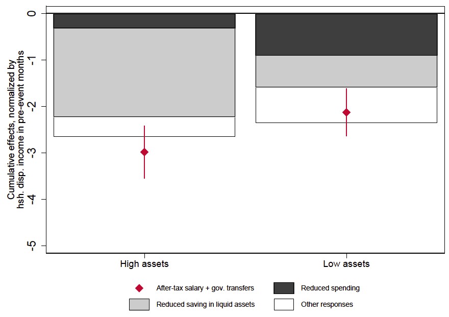
Notes: All outcomes measured relative to the household’s average disposable income in the months before the job loss. ‘High assets’ group consists of households with liquid assets worth at least two months of disposable income prior to job loss. ‘Low assets’ group consists of households with liquid assets below this threshold prior to job loss.
Concluding remarks
In summary, we find that household self-insurance makes up for 70% of the net income loss following job loss. Our analysis investigates the relative importance of the multiple responses underlying this result. Responses can be grouped into two classes of behaviour.
First, reduced saving in liquid assets and increased borrowing are pure consumption-smoothing responses that allow households to move consumption forward in time without changing overall consumption possibilities. Second, and in contrast, increases in spousal labour supply and private transfers from family or friends mitigate the impact of the shock by expanding the household’s overall consumption possibilities.
Our analysis shows that the first class of responses, in particular savings in liquid assets, is quantitatively far more important than the second type.
These findings have broader implications along at least two dimensions. First, the fact that the most important class of behaviour is an intertemporal shifting of spending opportunities suggest that households to a large extent perceive job loss as a transitory shock to income. Second, the prominent role of liquid assets in describing the response suggests that theoretical models that incorporate liquid savings can go far in capturing the most important self-insurance effect associated with job loss.
You can read more about the research in the CEPR discussion paper here
References
Andersen, A L, A S Jensen, N Johannesen, C T Kreiner, S Leth-Petersen and A Sheridan (2021), “How do households respond to job loss? Lessons from multiple high-frequency data sets”, CEPR Discussion Paper DP16131.
Basten, C, A Fagereng and K Telle (2016), “Saving and portfolio allocation before and after job loss”, Journal of Money, Credit and Banking 48(2-3): 293–324.
Cocco, J F (2013), “Evidence on the benefits of alternative mortgage products”, Journal of Finance 68(4): 1663–90.
De Nardi, M, G Fella, M Knof, G Paz-Pardo and R van Ooijen (2020), “Family and government insurance: Wages, earnings, and income risks in the Netherlands and the US”, VoxEu.org, 6 November.
Flaaen, A, M D Shapiro and I Sorkin (2019), “Reconsidering the consequences of worker displacements: firm versus worker perspective”, American Economic Journal: Macroeconomics 11(2): 193–227.
Ganong, P, and P Noel (2019), “Consumer spending during unemployment: positive and normative implications”, American Economic Review 109(7): 2383–424.
Halla, M, J Schmieder and A Weber (2018), “Job displacement, family dynamics, and spousal labour supply”, VoxEU.org, 13 December.
Jacobson, L S, R J LaLonde and D G Sullivan (1993), “Earnings losses of displaced workers”, American Economic Review 83(4): 685–709.
Jappelli, T, and L Pistaferri (2010), “The consumption response to income changes”, VoxEU.org, 2 April.
Landais, C, and J Spinnewijn (2020), “The value of unemployment insurance”, Review of Economic Studies (forthcoming).
McGarry, K (2016), “Dynamic aspects of family transfers”, Journal of Public Economics 137: 1–13.
Sullivan, J X (2008), “Borrowing during unemployment unsecured debt as a safety net”, Journal of Human Resources 43(2): 383–412.